Spatial Vision recently undertook some work which utilized the Python Whitebox toolset. In this blog, we will demonstrate what the toolset is and how it can be leveraged to perform hydrological modelling within Python.
What is Whitebox?
Whitebox is an open source toolkit developed by Dr. John Lindsay from the University of Guelph. Originally designed to be a plugin to support the Whitebox Geospatial Analyst Tool (Whitebox GAT), it became a standalone library able to be used in a wide variety of solutions including Python. Still actively being developed, it provides an MIT license which allows the toolset to be incorporated into other GIS software packages.
Demonstration
For this evaluation, we are using a 32bit floating point LiDAR derived DEM with a horizontal/vertical resolution of 0.2m/0.1m (find out more about our LiDAR data supply). The area of interest (AOI) is a section of the Plenty River located west of the Yan Yean Reservoir in Whittlesea, Victoria, Australia. Results are being displayed with ArcPro 2.6.
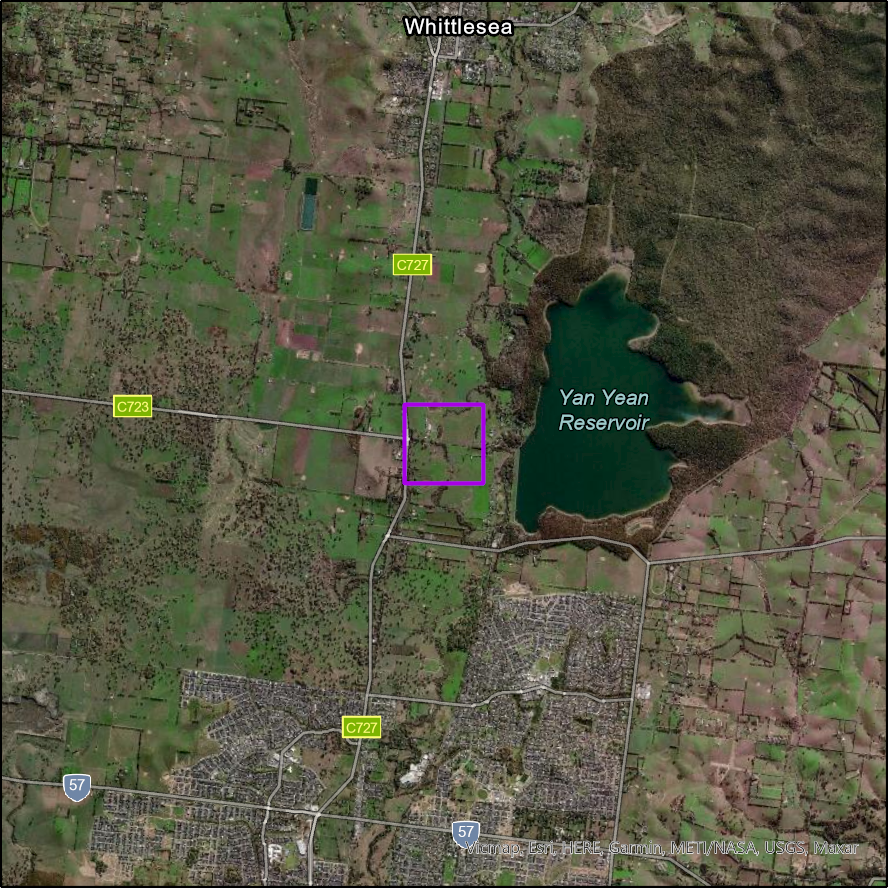
Figure 1 – AOI overview
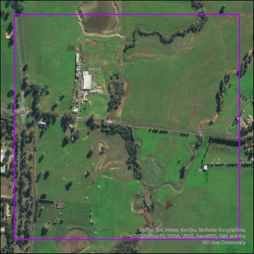
Figure 2 – AOI
The below table shows our program versioning and environment settings.
| Program/Module | Version |
|---|---|
| Python | 3.7 |
| whitebox (module) | 1.1.0 |
| ArcPro | 2.6.0 |
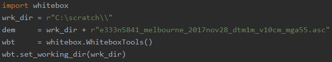
Firstly, lets setup our Python environment, set a few base variables and then inspect our DEM.
Before we commence our analysis however, we need to convert our raster into whitebox tools native elevation format called ‘.dep’. If the raster is not converted, it will result the tools truncating the raster data as an integer type and drastically affect the ability for granular details that can be obtained using floating point raster types.
![]()
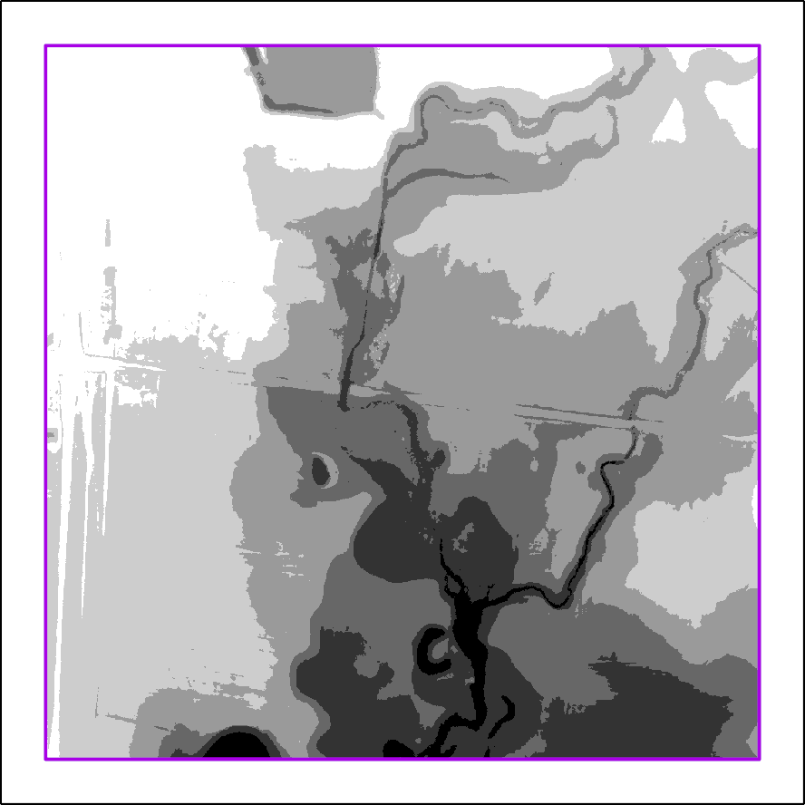
Figure 3 – Erroneous DEM when not converted to .dep format
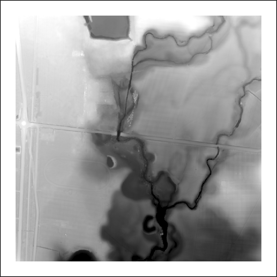
Figure 4 – Raw LiDAR DEM
On a first glance, the DEM looks just like any other DEM, but before we can sink our teeth into any hydrological analysis, we need to determine if the DEM is hydrologically enforced; that is to say, does it have sinks in the DEM. In order to determine this, we can use the sink function to output all known sinks in the DEM.
![]()
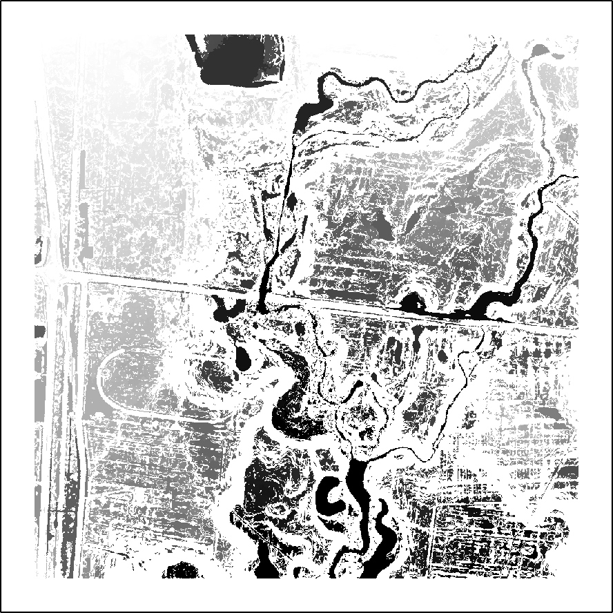
Figure 5 – Sinks within DEM
Just as we expect, the DEM is not hydrologically enforced as there are many sinks within the dem. We now have a decision to make on how to create the hydrologically enforced model. There is the typical ‘fill’ approach which will increase the sink values until they are just a little bit lower than their neighbouring cells, or we can take the ‘breach’ approach which will maintain the sink heights, but will build channels to cut through the DEM and make sure that all the depressions are connected so that every cell can flow into another cell. There is also a secondary type of breaching called ‘breach least cost’ which as it says, will breach the DEM with more control parameters based on the cost to breach the depressions. For the purposes of comparison, we will start with all three.

Note that with the above code we first applied a fill/breach action on individual pits. This acts to get rid of single cell depressions first before we fill/breach depressions that are larger than one pixel in size. This pit filled raster is then passed into the larger scale fill/breach function. The DEM may not appear significantly different after the single cell pit algorithms are completed, but the effect will be more evident once we proceed to the larger scale step.
We found the best result was found when using the breach_depressions_least_cost algorithm. It was able to effectively cut through road obstructions which would normally utilise culverts to channel water underneath them.
The best candidate can be seen when the Flow Accumulation function is run. We decided to include an iteration of the breach least cost where the ‘fill’ tag is not used in order to showcase the stark difference the use of this tag can have on creating a functional flow raster.

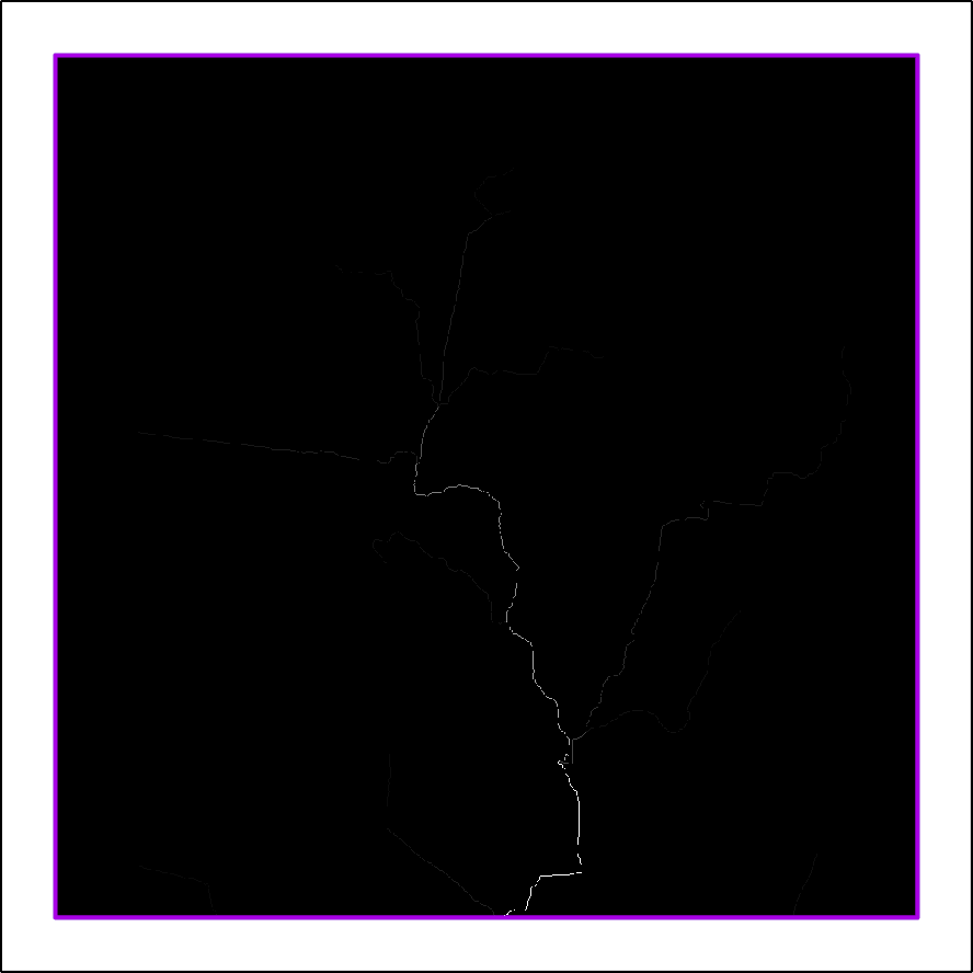
Figure 6 – Filled Accumulation
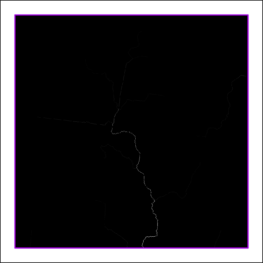
Figure 7 – Breach Accumulation
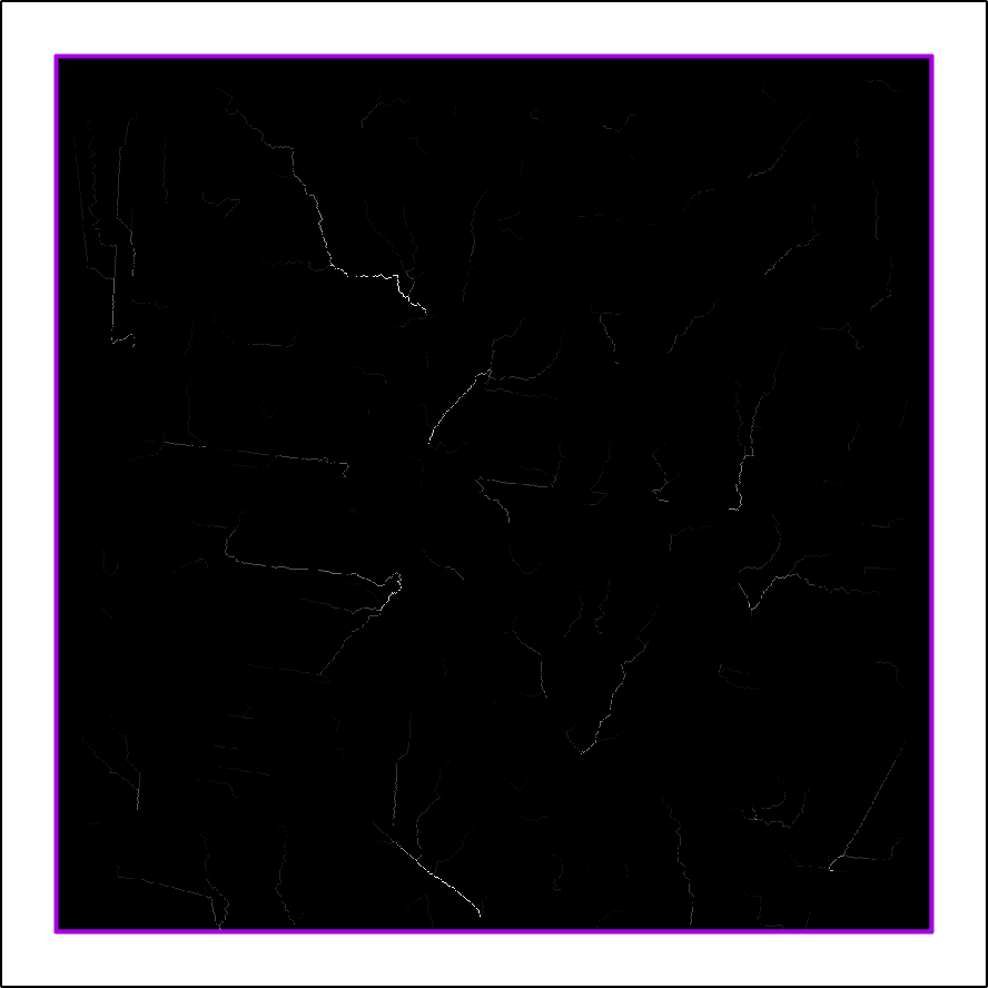
Figure 8 – Breach Least Cost Accumulation

Figure 9 – Breach least cost accumulation with fill tag
Now that we have created the accumulation rasters, we need to extract the pointer raster to determine flow direction of the raster.
![]()
With the pointer raster extracted, we can now extract the stream vectors from the DEM. This is three step process. First the Accumulation raster has a standard deviation contrast stretch applied to it in order to filter out small inconsequential streams. This leaves the main streams ready for extraction.

In order to extract the streams, we applied a standard deviation stretch to the flow accumulation raster. This acts to simplify the streams down into more manageable numeric categories. In this instance it applied a cell value of 7 to all background cells and anything larger was classified as a stream. This meant that only the major streams were extracted and turned into vectors. Upon comparison with existing VicMap data, we can see that there is a potential for correction to the existing dataset in this area.
Figure 10 – Breach types
Using the Whitebox toolset, we were able to programmatically import a DEM, hydrologically correct it to ensure flow and then extract new stream vector lines from it.
Whitebox has some great packaged tools to leverage and we highly recommend digging into it and having a play.
Resource: Whitebox Tools Manual

Figure 11 – Full script

Figure 12 – Full flow
- Case Study: GIS Service Plan - July 24, 2024
- Climate Change Statement - November 9, 2021
- Welcome Ryanne Firme – Digital Cadastre Modernisation Team - May 21, 2021