In these blogs (part 1, part 2), I take a look at GeoPandas and go through a worked example to show off some the cool things it does. To do this, I set up an Anaconda environment with Jupyter Notebooks (for doing a code demonstration) and of course GeoPandas and its dependencies.

Through my own unofficial observations (and this is no doubt true across industries), the dominant paradigm in spatial is proprietary software. Not just in terms what people use, but also what people are comfortable with. Open Source can be a bit intimidating, without all the gloss and advertising added by the big companies (case in point, ESRI). For this reason, it seemed worthwhile to go through the steps I took to set up this environment, so anyone can get into doing some Open Source spatial stuff.

Why Anaconda?

The answer to this one is easy – you basically have to use Anaconda to get the GeoPandas environment up and running. I believe you can technically get everything installed using the de facto python package manager pip, but unfortunately (and for a reason on which I’m not completely clear) pip is just not configured to install the dependencies for GeoPandas correctly. It takes some fiddling, and Anaconda does away with that fiddling, plus adding all the benefits it brings to the table.

Getting set up

1. Download and Install Anaconda
   • There are two options – Anaconda and Miniconda. Anaconda comes bundled with a bunch of science and research libraries (which we don’t technically need here), whereas Miniconda comes with just bare necessities.
   • Choose whichever you like (I used full-blown Anaconda for my demo), as the instructions will all be via the command line.
   • Note that Anaconda now comes with a flashy new GUI called Anaconda Navigator which simplifies environment management significantly, but we’re going to pretend it doesn’t exist!
   • Download and install Anaconda, or Miniconda – if you need help choosing there is a guide here
2. Create a new environment
   • Once installation has finished, we can create our environment
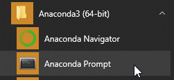
   • I did this install on Windows, and in Windows all of our commands need to be run through an Anaconda prompt. To start an Anaconda prompt, find it in the start menu under your Anaconda folder
     
     From a Mac, simply open a new terminal window
   • Run the following command to create a new blank environment called “geopandas-env”

     conda create --name geopandas-env

3. Install the dependencies
   • To work inside our new environment, we need to ‘activate’ it
   • You can see what environment you are currently in on the command line by the brackets at the start of the current working directory
     
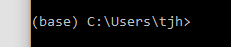
   • In our default Anaconda prompt, this is “base”, as above
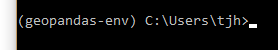
   • Run the following command to activate your environment

     conda activate geopandas-env

     The “base” from above should now read geopandas-env
     

   • Next, we need to add the appropriate package channel. Channels are the way that Anaconda manages its package repositories. The default conda channel does not have everything we need, but the community-supported conda-forge channel does. To enable the conda-forge channel, run the following:

     conda config --add channels conda-forge

   • With the conda forge channel added, we can now install GeoPandas. Conda prioritises its channels, and the conda-forge channel we just added is at the bottom of its list. This just means we need to tell conda to look on the forge channel for GeoPandas, using:

     conda install -c conda-forge geopandas -y

4. Creating a Notebook
   1. Finally, I want to create some Jupyter Notebooks to demonstrate GeoPandas using the new environment we’ve made. Jupyter comes installed with Anaconda, but to use it with the new environment we’ve created, we need to install the Jupyter kernel in our environment. Do so with the following command:

      conda install nb_conda_kernels -y

   2. Once this has completed, we can spin up a Jupyter Notebook. I recommend changing the directory to where you would like to keep your notebooks at this stage, for example:

      cd C:\Projects\geopandas-project\

   3. Then we can spin up a notebook instance by running:

      jupyter notebook

   4. Pro tip – if you want to access your notebook over a network (for example, if you want to use the notebook on another local computer), you can specify the ip address and port as follows:

      jupyter notebook --ip 0.0.0.0 --port 8888

      You can then access the notebook at your local ip or network name

   5. the default http://0.0.0.0:8888 address will not work with this option, change it to:
      http://localhost:8888
   6. Having started the notebook from within our environment, we can create a new notebook directly in the environment using the “Python 3” option.
      
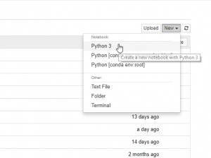
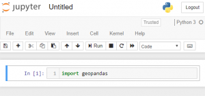
      If you have other environments with notebook kernels, we can access these here too.
   7. Create a new notebook, and try importing geopandas. If the line of code runs successfully, you’re ready to go!
      
5. Replicating your environment
   • Now that you’ve set up an environment, we can save out the settings to an environment yaml file that we can use later to replicate it. From within your environment, the following command will dump your settings to an environment.yml:

     conda env export > environment.yml

   • You can then create a new environment by running the following command

     conda env create -f environment.yml --name

     ---

     That’s it for the Python Insights blog series! We hope you have enjoyed these tutorials and have learnt some skills that you can apply in your own workplace.

     For more Python, check out our Geopandas tutorial here.
     For further information, please contact Spatial Vision at info@spatialvision.com.au