Before we begin, I would like to start this article with a handful of prefacing caveats:
- This blog relates to the use of Geospatial data in modelling different real world scenarios
- Most of this article has been written from an ESRI use-case point of view. This is not to say that it can’t be reproduced in another GIS platform, but I’ll leave that to you to try, inspired reader!
- Any processing route I have taken is probably one of many options that can be followed. In the world of GIS, as in many endeavours, there are many (deep) rabbit holes an analyst can dive down, so follow the white rabbit at your own peril!
- This blog is not a discussion on Monte Carlo simulations, machine learning, or any other intense modelling technique. This is more a cursory level exploration of an interesting GIS problem and how we may go about solving it.
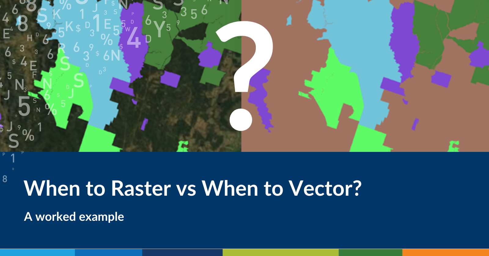
To raster or to vector
I was recently working on a logic problem for a client which entailed looking at the amalgamation of multiple spatial features into a unique layer. This was one stage of a larger framework, but one that saw me going deep down a rabbit hole of raster vs. vector musings.
The crux of the issue was that we wanted to know unique combinations between several layers—some raster, some vector—and then determine what these unique combinations represented while retaining a relational linking ID before applying back to a separate master raster.
Given that the final stage was to apply the output back to a raster, it did imply that anything produced had to be converted back into a similar grid format at the final hurdle. But all the pre-work could be done in whatever format we wanted. That being said, to avoid the hassle I used raster throughout.
This was not a problem of raster maths, fuzzy analysis, Bayesian modelling or some other complexing modelling technique – it was more an exercise of clever GIS tool application using some logic and simple precepts. It’s true – not everything requires a machine learning algorithm. Sometimes lateral thinking and a simple approach can be just as satisfying.
Now, like any long-term worker in the GIS industry, I have developed an affinity to one data form over another – raster in my case. But, this problem allowed me to explore comparable methods in both formats and explore what outputs would look like on both sides of the fence in order to assess on which side the grass is actually greener.
Raster to polygon conversions
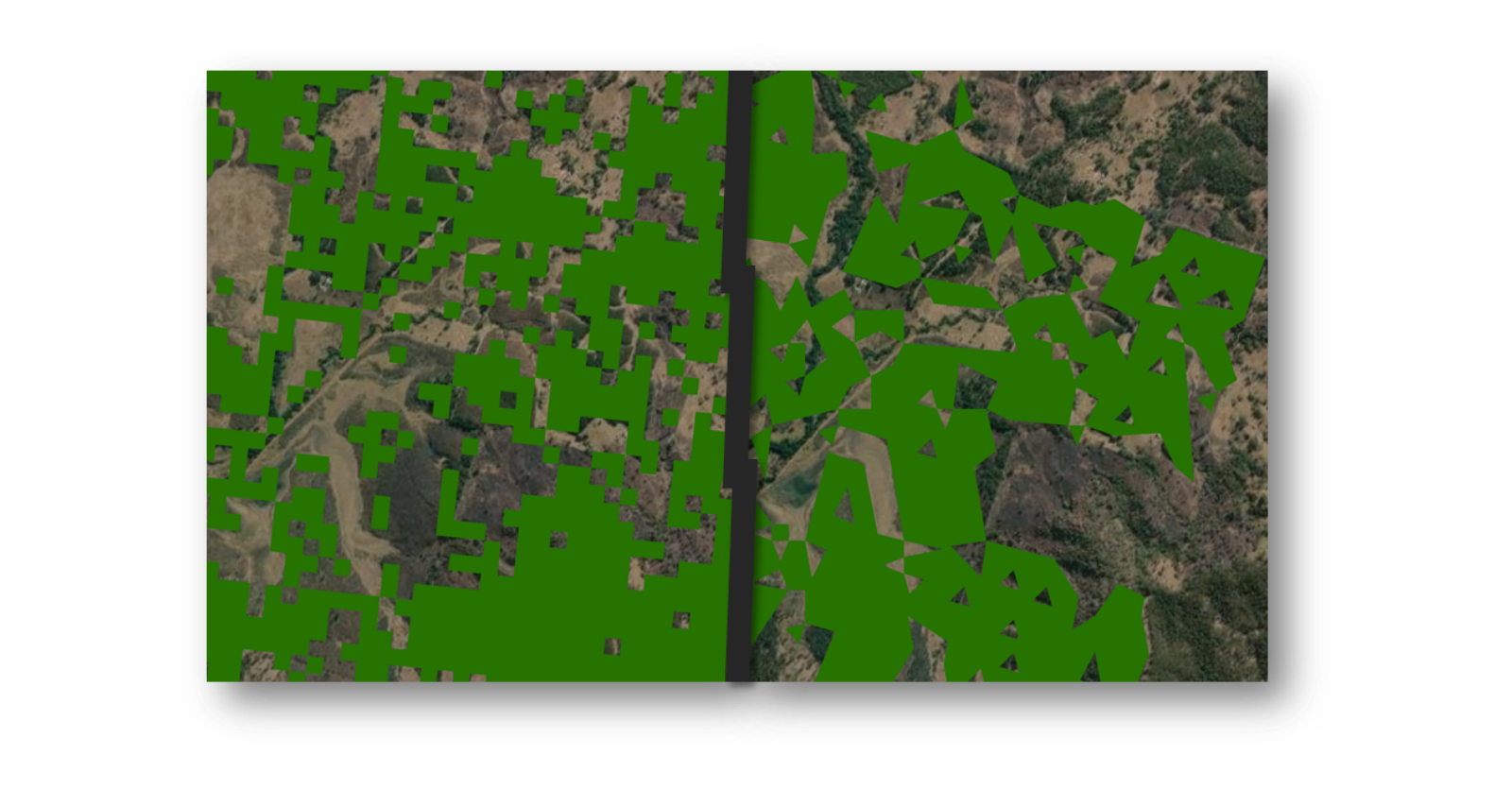
I’m not going to dive into a conversation on data resolutions, projections, snapping and other pre-processing matters – let’s assume everything is above-board on that front. However, I do want to briefly discuss raster to polygon conversions and why they produce ugly-looking vector data outputs.
Rasterised polygons often get used incorrectly by inexperienced analysts and cause more issues than they solve. Plus, aside from cases where the outputs are all generated from the same resolution and are all snapped and aligned, I have never come across a use case where this was a necessary endpoint. There are more elegant solutions to bring raster data into a polygon format (and don’t get me started on simplified raster-to-polygon conversions… those little triangle outputs are the bane of my existence!).
There are notable exceptions, of course – fishnets or polygrids are perfectly acceptable analysis outputs. But a raster is not a polygon. There are better ways of outputting or embedding raster data into a vector format.
Rasters vs. Rasterised Polygons
Now, in contrast to what I actually had to work with, for the sake of this exercise let’s assume we have two sets of comparable datasets: one presented as raster, and the other as vector. Assume there are three main themed layers representing local government areas, national park locations, and land tenure boundaries.
Combine vs. Intersect
The first comparison I explored was the raster spatial analyst tool Combine versus the vector analysis tool Intersect. Both these tools find the unique combined value between two or more layers, but only where there is an actual intersect between all input layers. This is an important distinction for both tools: the output will only be for where each input layer interacts; if you have two inputs, this will be where each layer touches each other; if you have three inputs, it will be where all three layers overlap, and so on. Therefore, outputs can be quite small or non-existent if there are no unique combinations.
What is the Intersect tool?
The vector based Intersect tool produces a useful output which retains the attribute fields from each input, including the object ID for each relevant input as well as a unique object ID for the intersection output. This way you can neatly trace back what categories underpin each layer of the input and use the unique ID to link a record back in any further analysis.
An honourable mention should be given here to the Spatial Join tool. Spatial Join only allows for two inputs: a target layer and join layer. The target is the coverage into which you want to look at joins or intersects, and the join layer is the layer to append into the feature layer. As only the target layer geometry is retained, it is similar to the Intersect tool, but it does allow for a more varied range of matching options, search distances and join types.
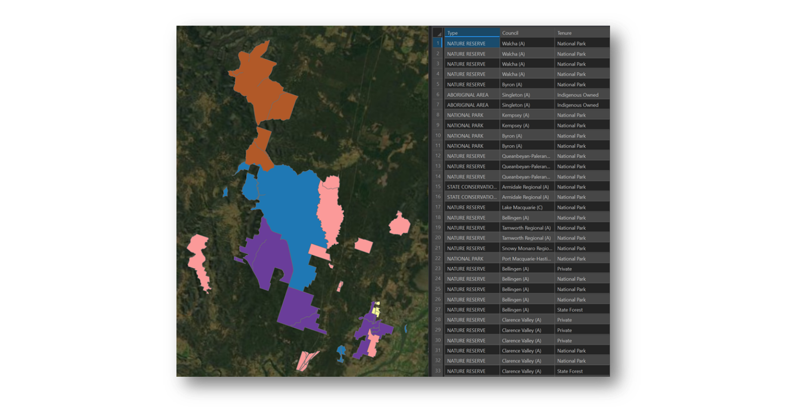
Intersect tool output using Council, Tenure and National Parks
What is the Combine tool?
The raster-based Combine tool produces an interesting output for further use in analysis. As with any raster analysis, the Value field from each input is used, so any supporting attribute information is not carried through. However, the Combine output creates a new Value record where there is a unique overlap and then appends on a supporting attribute field showing the Value record of each supporting input layer. So, if there were three inputs, there would be three supporting fields for each of these – one for Local Government Areas, one for National Parks and one for Tenure. This way, with a Combine output, there is a method to allow relational links to be established from output to each supporting input.
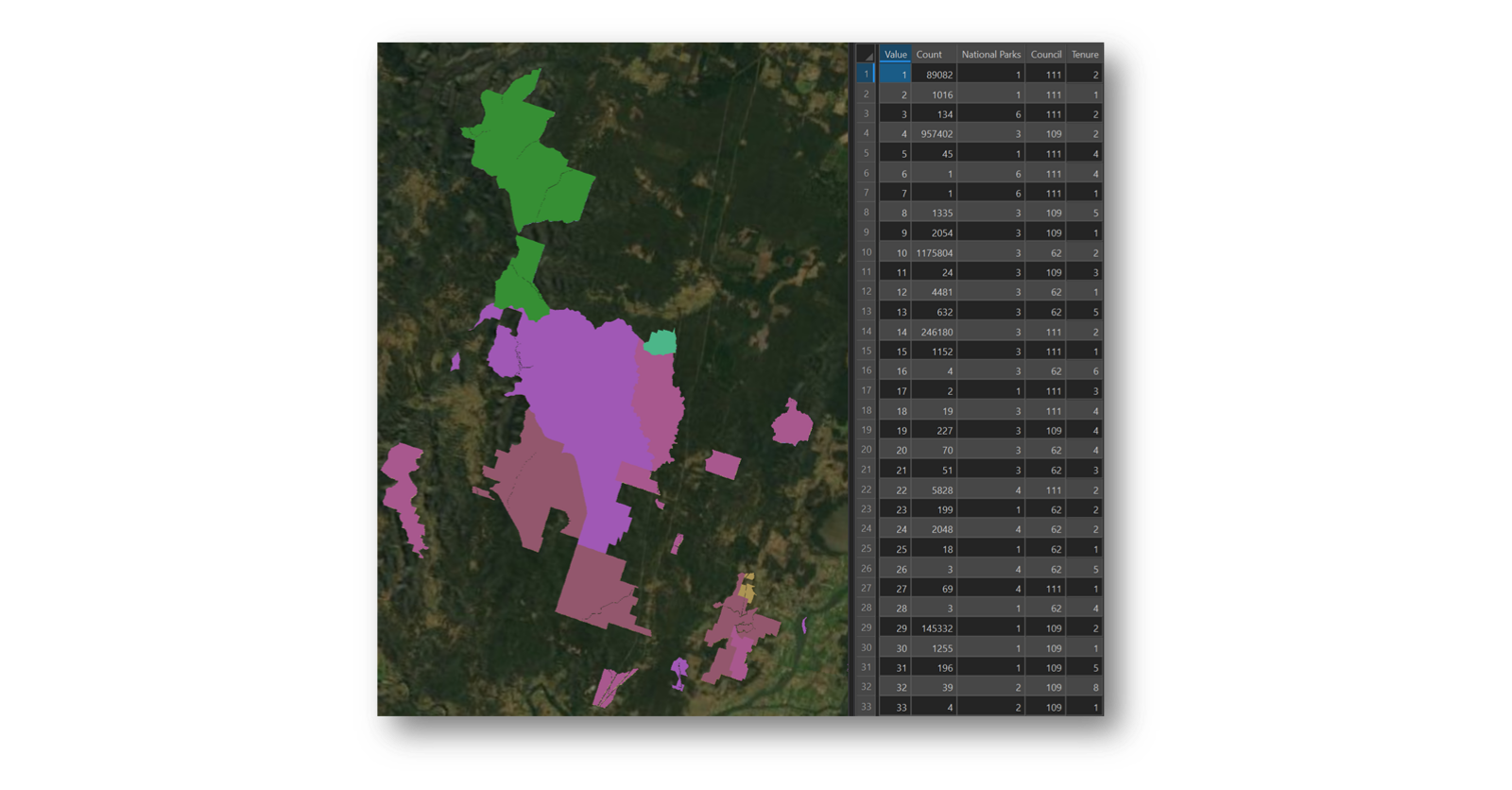
Combine tool output using Council, Tenure and National Parks
Also, interestingly, the output pixel depth and type are adjusted accordingly for however many unique combinations are created. I initially started out with two 4-bit unsigned inputs and an 8-bit unsigned input and ended up with a 32-bit unsigned output. Overkill for my use case, but it was handy to know that I did not need to worry about depth and type.
The pitfalls of Combine and Intersect
However, a downside of Combine is that there is a default limit on the output to 65,536 unique combinations. This can be adjusted within Arc settings, but there is the question on who would actually need so many combination values? In comparison, intersect does not have this limit, it is only limited by the usual bounds of a shapefile or geodatabase feature layer output.
As I have mentioned, the big downside for either Intersect or Combine is the fact that it only accounts for combinations where there is a unique overlap between all input layers. In my use case, I was also interested in retaining all other data where there was no unique overlap. So, with three inputs, I was also wanting to look at cases with only 2 overlaps, or also areas where there was no overlap at all between all inputs. In essence, I wanted to retain the No Data points and reflect this back in an output.
Given this consideration, there are several steps that are necessary for processing in raster format. Before delving into that side, it is useful to reflect on the vector view of the world and comparisons that can be drawn.
How does vector compare to raster?
One of the cornerstone GIS Analyst tools when interrogating multiple data layers is Union. This allows for the unique combination of multiple data layers, regardless if there are intersections or not between the input layers. In my use case, this is a very big benefit as I can quickly throw together several layers and throw out an output that can show where intersects exist and where there are none. Ideally for my overall problem, it creates unique geometries for all intersecting areas and joins all relevant values from all contributing layers into that geometry.
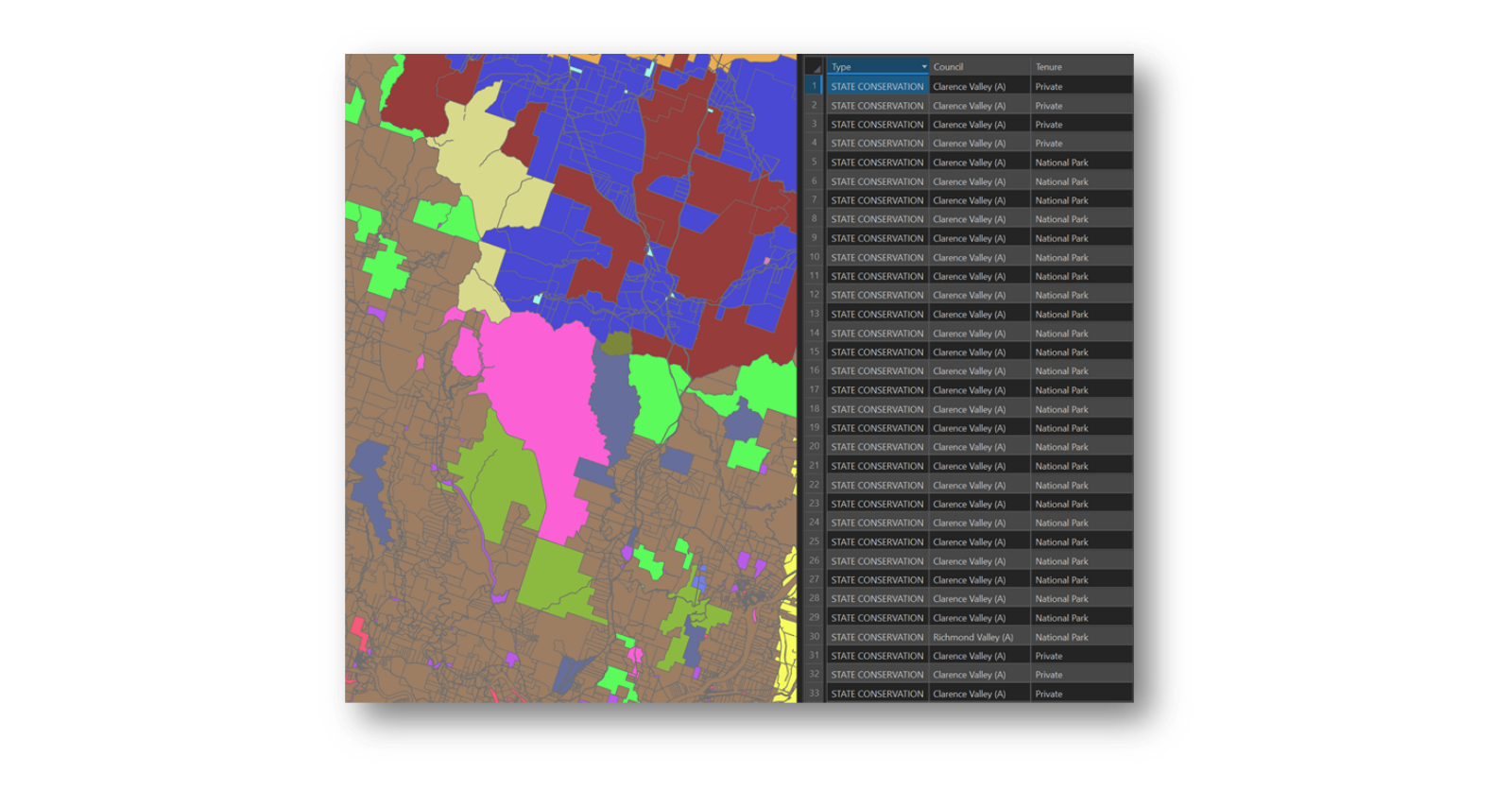
Union tool output using Council, Tenure and National Parks
The attribute table for a union output will contain all relevant attribute fields from every input. If a field name is duplicated, then the duplicate will be renamed accordingly. What is handy about how the attribute table is structured is that if there are no intersections between layers, then values are retained for at least one of the inputs, and all other fields are given a blank value, which helps identify non-overlaps. If there are overlaps, then all relevant field entries are retained. In this manner the unique values and combinations can be determined.
Honourable mentions should be given here to the Merge tool, a useful tool in the space of joining several layers, but not useful in my particular case. Merge can join several layers, but it preserves the geometry of every input and does not create unique intersects. Therefore, if there is an intersect, there will be overlapping geometries in the output and no unique combinations are created.
Conducting the raster analysis
To undertake the raster side of this analysis and processing, I first created a full area of interest zero-value raster to account for the full analysis extent and any potential No Data regions. This zero-value raster could then be joined to all inputs. To undertake this join, I made liberal use of the Mosaic to New Raster tool as this allows for multiple raster inputs to be joined. There are many ways this tool can be used to join raster layers together. But in my case, to create a continuous coverage, it was of particular use as it could fill in those No Data areas in my full area of interest.
If I was to concentrate on a more mathematically minded output, then I would consider Cell Statistics, as this tool can run a number of statistical analyses on a cell by cell basis. But all I was concerned about was joining multiple rasters together without a care to the mathematical validity of the output.
A few fundamentals of the Mosaic to New Raster tool. First to consider is the bit depth of the input and output. If the combination of the two rasters will create a new value range that extends beyond the default pixel range (8-bit unsigned), then consider selecting a new bit depth pixel type. This is particularly true if we are to deal with negative numbers or floating-point numbers.
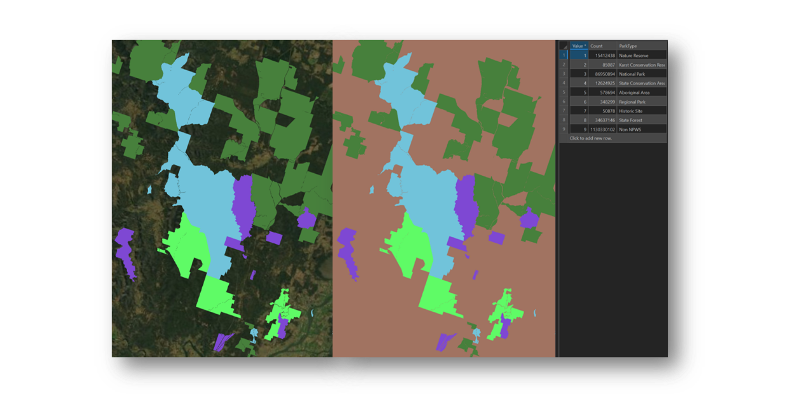
National Parks raster, before (left) and after (right) Mosaic to New Raster operation with a zero-value base layer
Second is the cell size, or resolution of the outputs, typically this tool defaults to the resolution of the first input raster. But in my experience, this can be a bad assumption to make. If there are mismatching projections or grid sizes, it is best to first make sure all the inputs are in a comparable spatial reference, then force the cell size and specify a value (and in good practice, try and set the spatial reference as well).
Third is to consider the Mosaic Operator, the method used to mosaic overlapping cells. This is key to my problem at hand. Similar to Cell Statistics, there are a number of simple statistically based operations, such as maximum or minimum value. But for my use case, I concentrated on the First and Last operators. As with most multi-input tools, there is a perceived hierarchy of inputs, therefore the first input in the list is processed first and the last is done last. If we want to preserve the values of the top most input and append on No Data, or zero values from the full area of interest raster, then the First operator should be used. By default, Last is always selected, so this needs to be checked.
Like any good raster analysis tool, Mosaic to New Raster only cares about the Value field in any given raster. Any descriptive attributes are ignored. Hence, once the tool is run, all extra descriptive fields in the input raster (if present) are not carried through to the output. If you want to re-join any descriptive attributes, you will need to append back on after the fact.
With all these concerns in mind, I was able join the full extent zero-value raster to all my base inputs to create full coverages for all input rasters. Then using these outputs as inputs, I re-ran the Combine tool as outlined earlier. The difference now is that I was able to get combinations for areas where, technically, No Data exists.
Pulling it all together
The final step was to trace back the value fields for the three inputs – Local Government Areas, National Parks and Tenure – and provide a descriptive value against each unique value input for the three inputs. Using the three supporting fields for each of the inputs as an ID, I quickly created three descriptive fields, formed a relational link between input value and output ID link and copied across the values.
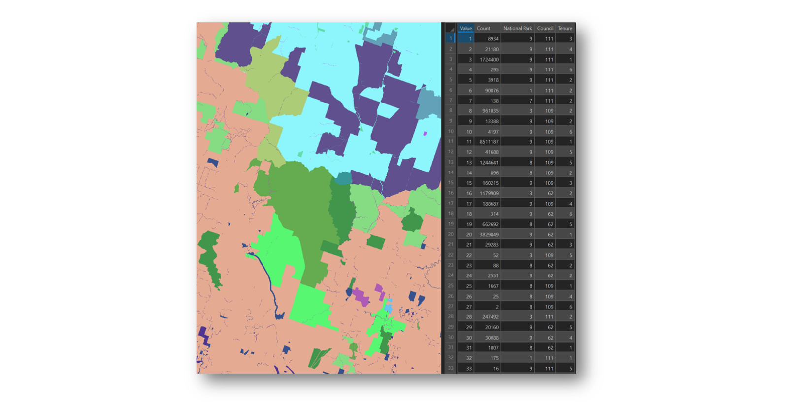
Final Raster output combining Council, Tenure and National Parks with zero-value base layer
The final product was a full area of interest raster grid that could identify, for any given cell, what the unique combination of values were, even if one had no data within that cell. This I was able to apply back against various other raster grids, pull out some useful metrics and analyse in secondary platforms such as in Excel Pivots or Power BI.
Of course, my final product did push past this three-input scale and ended up having twelve inputs and nearly a quarter of a million unique combinations, rendering the Combine tool obsolete. But “How to push past the Combine limits” can be a discussion for another blog – these fundamentals are essential to lay out the ground work.
Hopefully you found these musings helpful, and my journey down this GIS rabbit hole has saved you going down yet another.
If you have any questions, free to reach out here, or connect with me on LinkedIn.
Harmen is a skilled analyst and modeller with over 6 years of experience in Geospatial Analysis.He has a strong background in the ArcGIS environment, Python scripting and the application of automation in modelling processes for large datasets and series.This has most recently been applied in the evaluation and processing of environmental works program data across Victoria for the analysis of works size and alignment to best management practices.
- When to Raster vs When to Vector? A worked example - May 4, 2022
- Mapping the Future of Farming - August 9, 2019
- Great Ocean Road Erosion Impacts - January 10, 2019